November 4, 2024

`Bonding Curves: A Universal Tool for Building DeFi Protocols`

catslovefish.eth November 4, 2024

Abstract. Bonding curves, traditionally used to define the relationship between the price and supply of an asset, can be extended beyond their original purpose to serve as a universal tool for building decentralized finance [1] (DeFi) protocols. This paper explores how bonding curves can be tailored to meet the diverse requirements of various DeFi applications — including token swaps, fair launches, prediction markets, lending markets, and more — beyond the conventional scope of Automated Market Makers (AMMs), which are mainly for token swaps. By abstracting the mathematical principles of bonding curves, we demonstrate their ability to form relationships and algorithms linking any set of variables, thus serving as a universal tool within DeFi.*

1 Introduction

Decentralized Finance (DeFi) represents a transformative shift in the financial landscape, leveraging blockchain technology to create financial systems that operate without traditional intermediaries. This movement aims to enhance financial accessibility and efficiency by providing decentralized alternatives to conventional financial services. By enabling peer-to-peer transactions and automated processes, DeFi opens up opportunities for innovation in various financial applications.

A pivotal innovation within the DeFi ecosystem is the Automated Market Maker (AMM), which facilitates trading and liquidity on decentralized platforms. However, the application of AMMs has largely been restricted to token swap scenarios, which limits their flexibility and the breadth of financial services they can offer. A critical challenge remains: the development of a universal mechanism that can adapt to a diverse array of financial use cases beyond simple token swaps.

Bonding curves* [2] [3]* offer a compelling mathematical framework that articulates the relationship between an asset’s price and its supply. Originally designed for token sales and fundraising — ensuring continuous liquidity and predictable pricing without centralized control — the potential applications of bonding curves extend well beyond these initial uses. By customizing the parameters of bonding curves, we can cater to the unique requirements of various DeFi protocols, positioning them as a universal tool in the decentralized economy.

This paper investigates how bonding curves can evolve from their traditional roles to encompass a wide range of DeFi applications, including fair launches, bonding curve liquidity pools, prediction markets, and more. We present a comprehensive “zoo” of DeFi use cases where bonding curves can be effectively implemented. Through mathematical representations and illustrative examples, we demonstrate how these curves can be tailored to meet the specific needs of different protocols, thereby simplifying the design of complex financial systems and fostering fairness, efficiency, and innovation within the decentralized economy.

Furthermore, we propose a universal framework for constructing DeFi protocols that includes defining objectives, identifying counterparties, establishing clear functional relationships between parameters, and creating specific incentives and disincentives to ensure effective operation. This approach capitalizes on the adaptability of bonding curves, enabling their application across a diverse spectrum of financial scenarios and even decentralized societal frameworks.

2 A Zoo of DeFi

In this section, we present various use cases within decentralized finance (DeFi) to illustrate the versatility of bonding curves and provide clearer intuition on how they can be tailored to meet the unique necessities of different applications.

2.1 Fair Launch

In a fair launch scenario, a new token is introduced to the market without any pre-mining or early access for specific investors. Bonding curves can facilitate fair launches by providing a transparent and algorithmic method for pricing tokens based on supply and demand dynamics.

Mathematical Representation and Token Purchase Mechanics In the bonding curve model, the price p(sA) of a token is a function of its total supply sA. A simple quadratic bonding curve can be expressed as:

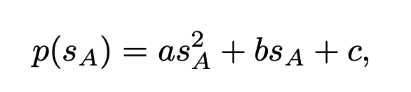
(1)

where a, b, and c are constants chosen to shape the curve appropriately. When a participant wishes to purchase an additional ∆s tokens, the total cost C is calculated by integrating the price function over the desired token quantity:

This ensures that each token purchased reflects the current supply and its effect on the price, accounting for the price increase as the total supply grows.

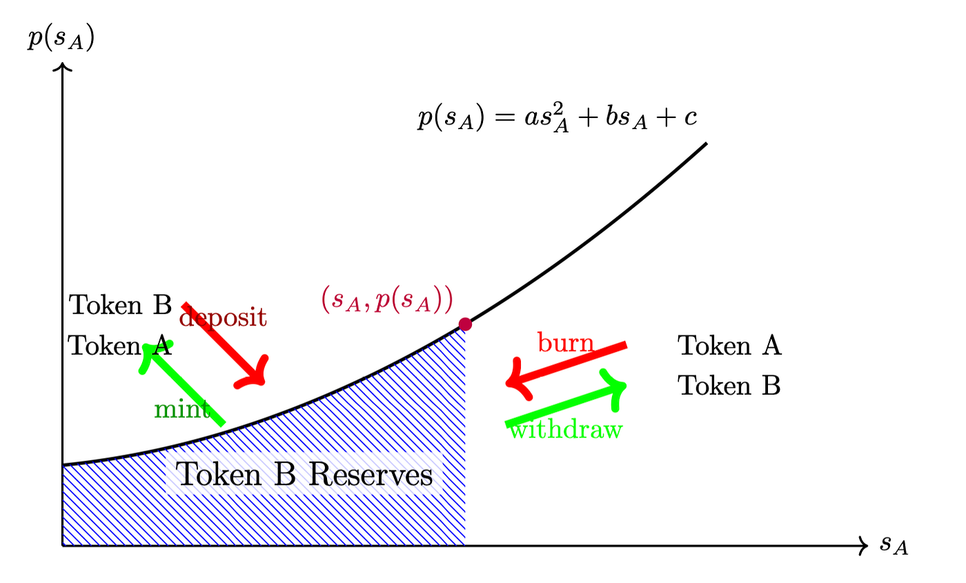
Figure 1: Illustration of the bonding curve for a fair launch, showing the relationship between the supply of token A and its price. The reserve of token B is represented as the area under the curve.

2.2 Dynamic Token Distribution

Bonding curves play a crucial role in enabling dynamic equity distribution within decentralized organizations. These curves provide a mechanism for contributors to earn ownership in proportion to their contributions, making the distribution process transparent and aligned with individual inputs.

Dynamic Tax Rate: Importantly, bonding curves do not always follow the same path for buying into and selling out of the token economy. The structure of these curves can be adapted to meet the specific goals of a project. For example, certain projects may require continuous inflows of capital to cover operational costs, such as daily expenses or contributor salaries, as well as investments for future growth initiatives.

By adjusting the tax rates or other parameters across different stages of token distribution, projects can ensure that early investors, crossover participants, and later-stage participants are treated equitably, while also supporting the project’s long-term sustainability.

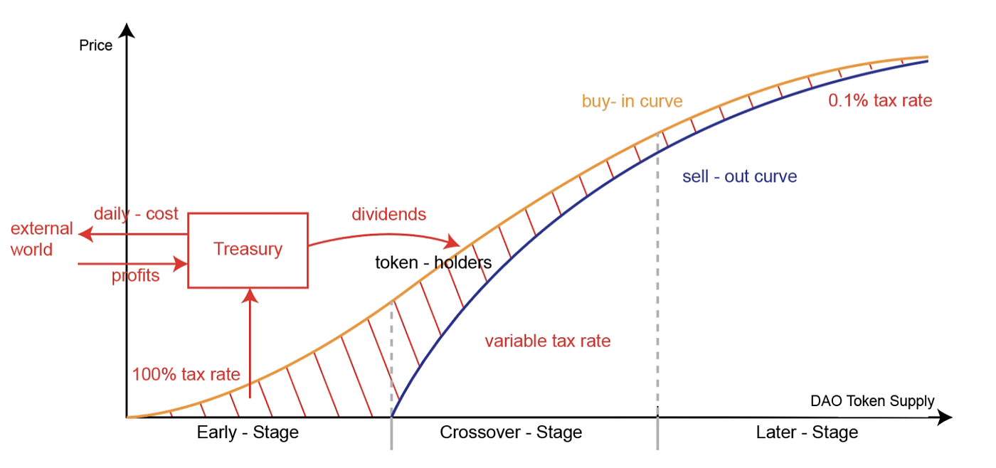
Figure 2: The tax rate transitions smoothly from a higher rate in the early stages to a minimal rate at later stages, ensuring sufficient funds flow into the treasury during times of high capital needs, while providing more liquidity for later participants.

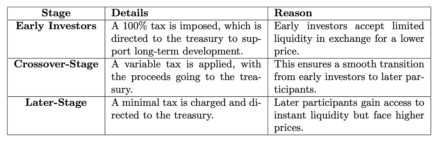
Table 2: Stages of Investment with Corresponding Details and Reasons

Hook: In some token distribution models, a dynamic condition or “hook” can trigger a significant event once a certain target is reached. For example, in a lottery-style distribution, once a predefined funding goal or target is met, a mechanism could be activated where the remaining tokens are randomly redistributed among all participants.

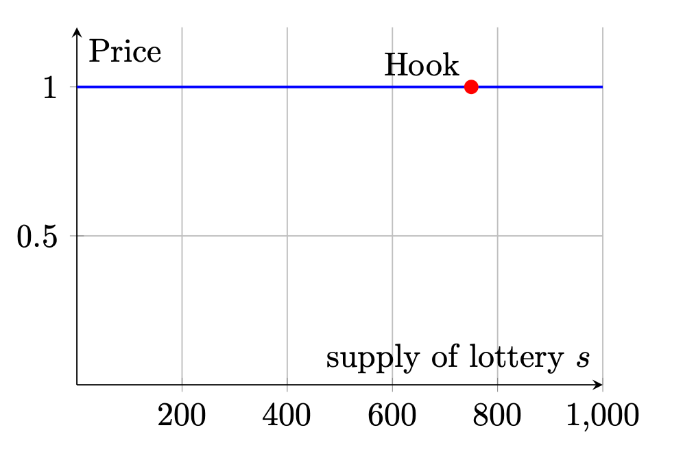
Figure 3: Hook Mechanism: Once the token supply reaches S = 750, the hook triggers a redistribution event.

2.3 Token Swap

In DeFi, token swaps allow users to exchange one token for another without intermediaries. AMMs like Uniswap determine the swap price based on a function of the reserves of each token in a liquidity pool, specifically using the constant product formula. While Uniswap does not explicitly use bonding curves that map price to supply, we can explore how bonding curves can serve the same purpose through a different approach.

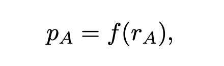
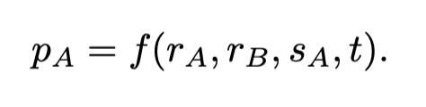
Bonding Curve as an Alternative Approach Traditionally, bonding curves map the price of a token to its total supply. In the context of token swaps, we can consider a bonding curve that defines the relationship between the price of token A and its reserve r_A in the pool, effectively mapping *p_A(r_A)*.

Mathematical Representation Consider a bonding curve that relates the price of token A to its reserve r_A:

(2)

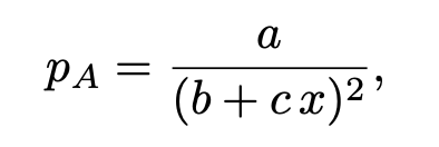
where f is a monotonically decreasing function, reflecting that as the reserve of token A increases, its price decreases. For a start, we can define the bonding curve function as:

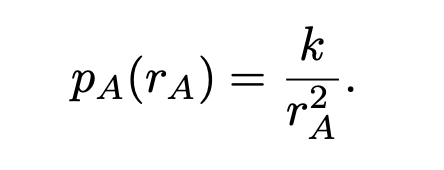
(3)

This equation implies that the price of token A is inversely proportional to the square of its reserve.

Deriving the Constant Product from the Bonding Curve

Starting from the bonding curve p_A(r_A) = k/r_A², we can express the reserve of token B as:

(4)

where C is the constant of integration. Assuming C = 0 for simplicity, we have:

(5)

This derivation shows that the constant product formula used by Uniswap can be obtained from a specific form of a bonding curve, bridging the two approaches.

Swap Mechanics When a user wants to swap ∆r_A amount of token A for token B, the reserves update as:

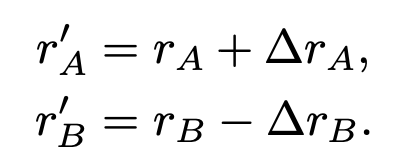
(6, 7)

Using the bonding curve, the amount of token B the user receives is:

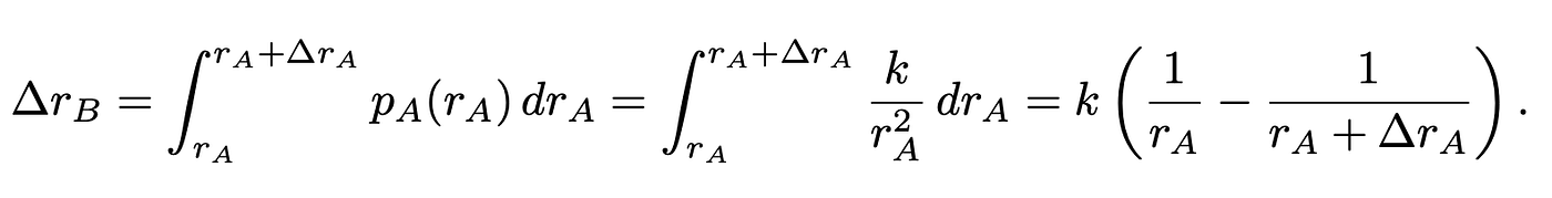
(8)

This result reassemble the swap mechanics in Uniswap, demonstrating that the bonding curve approach can replicate the same pricing and reserve adjustments.

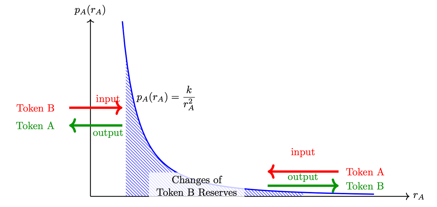
Figure 4: Illustration of the bonding curve for a token swap, showing the relationship between the reserve of token A and its price. The changes in the reserve of token B are represented as the area under the curve.

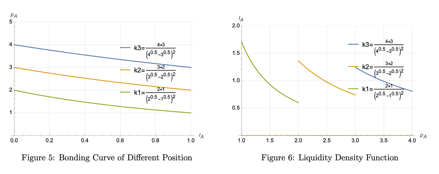
Discrete Liquidity Position

In a discrete scenario like Uniswap v3*[4] ¹, each liquidity provider has a unique position defined by a specific price range and associated liquidity parameter k, k can be determined by r_A*,r_B , p_small and p_big , where we set

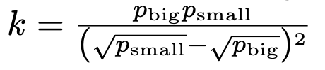
to fix r_A=1 when r_B =0. (In principle, we don’t need r_B , we only need ∆r_B )

¹ This discrete price scenario is effectively equivalent to the Uniswap v3 mechanism. In Uniswap v3, the liquidity density is plotted using parameters √p and virtual reserves(that is why it look like a line ), rather than the price itself. It’s important to be mindful of this distinction when comparing or analyzing similar systems.

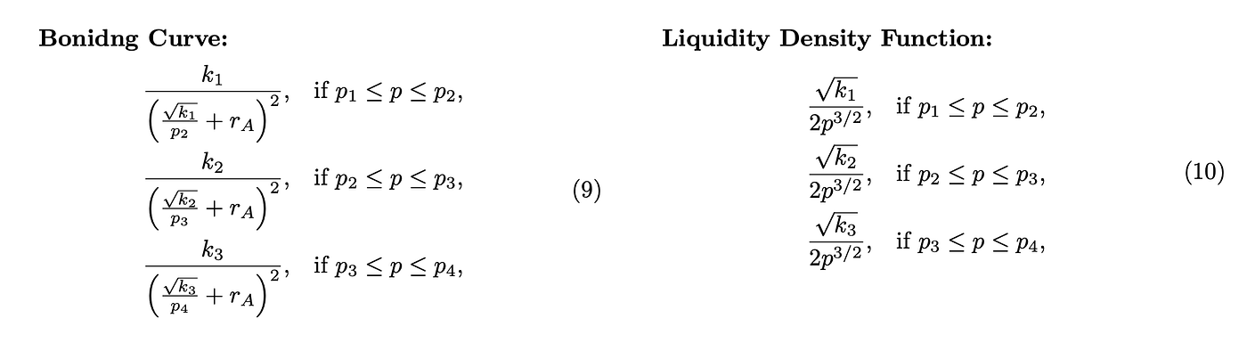
Dynamic Liquidity Distribution Imagine we aim to provide an arbitrary liquidity distribution based on a target, similar to Market Value Management. In Uniswap v3, this requires frequent liquidity adjustments (adding and removing). However, we can achieve a similar effect more efficiently by adopting a bonding curve approach, where we dynamically set and adjust the price range. This allows for smoother control of liquidity without discrete steps, essentially benching the bonding curve and set different range to meet the desired distribution more seamlessly.

we can set the bonding curve as

(11)

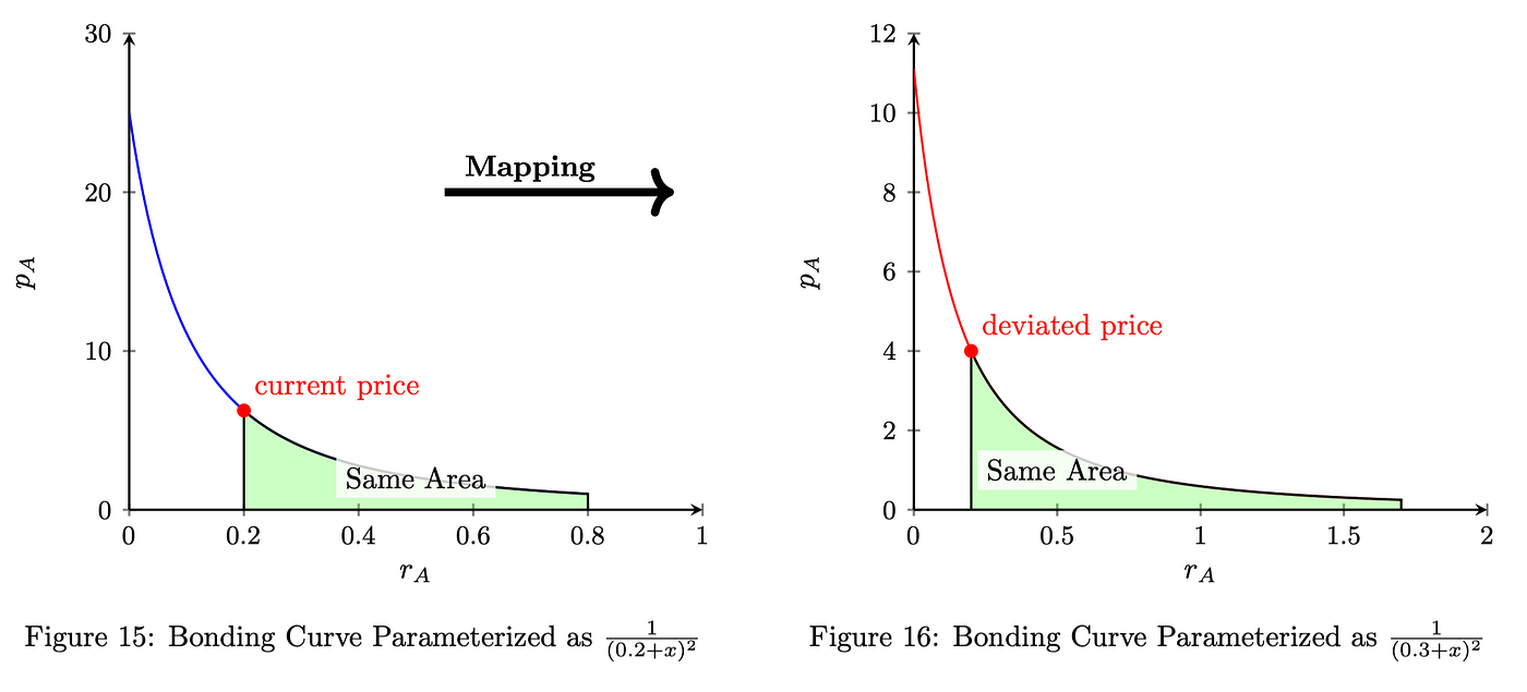
as long as it decreases monotonically and always > 0 Partial Remove Liquidity of Token B When the price of token A go up, we can partial remove some token B out of a position, this is essentially cutoff the bonding curve into a new r_A domain

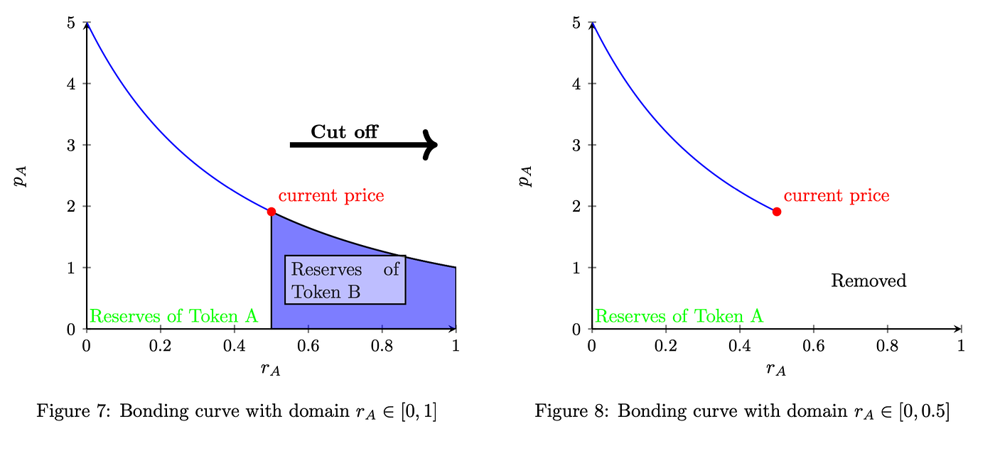
Partial Remove Liquidity of Token A When the price of token A go down, we can partial remove some token A out of a position, this is essentially cutoff the bonding curve into a new r_A domain

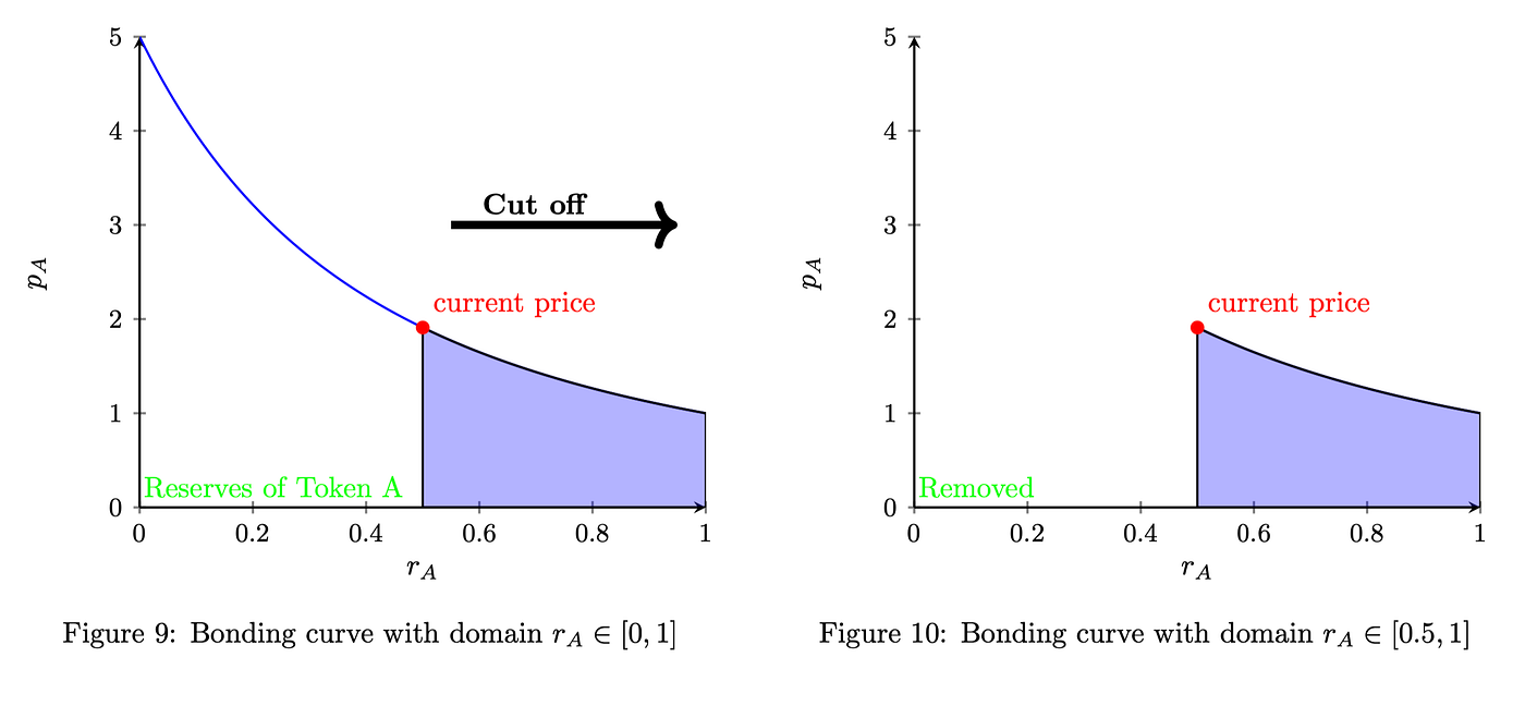
Liquidity Redistribution Outside the Current Price By ensuring that the integrated area remains the same for a given domain of r_A, we can re-distribute liquidity positions with the same token reserve A or token B across a price range that is outside the current price as p_a ∈(0,p_small) ∪(p_big ,∞)

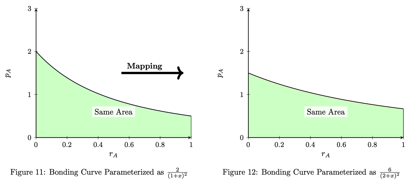
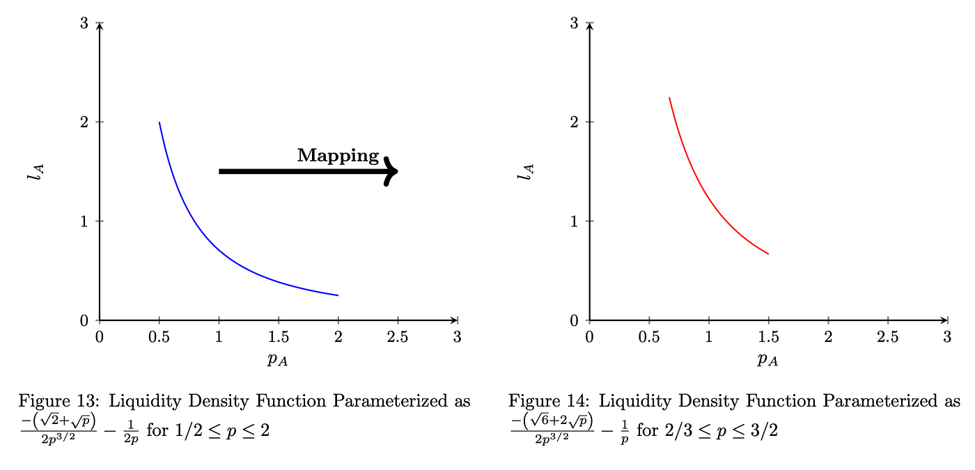
Liquidity Redistribution within the current price Reallocation of liquidity becomes slightly messy when p_A ∈[p_small,p_big ]; Still, as long as we keep the r_A and r_B within the position is equivalent after mapping, it doesn’t against anything².

Conclusion

Bonding curves can resemble the Uniswap and go beyond of constant product formula.

² An entry do not have to set the mapping price as the same price of current price, they have the freedom to enjoy the immediate Impermanent Loss. However, if the bonding curve is universal for all participants, then, the deviated price must equal to current price.

2.4 Extended Token Swap

In the context of decentralized finance, a token swap typically follows a specific bonding curve or pricing function, such as those used in AMMs. To extend beyond the conventional token swap mechanisms, we can explore more generalized forms using asymptotic analysis.

A rational function, defined as the ratio of two polynomials, can be used to model a broader range of token swap behaviors. Consider the following general relation for the price of token A, denoted p_A, as a function of its reserve r_A:

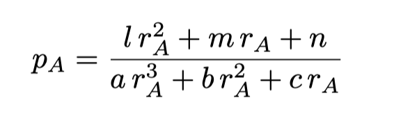
with asymptotic behavior as r_A → 0, p_A → n/cr_A and *rA →∞*, pA → l/ar_A

This rational function provides flexibility for modeling different price dynamics analytically. For reserve curve:

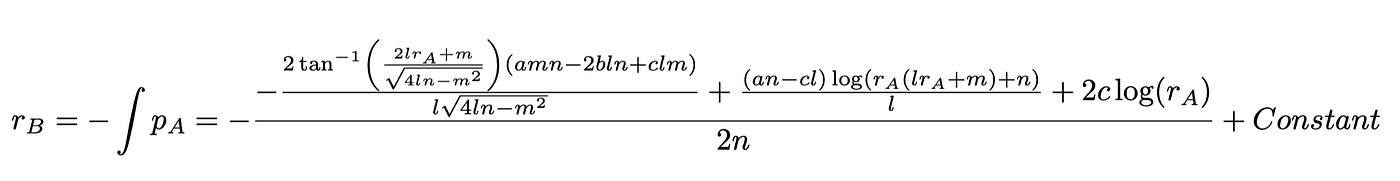
(12)

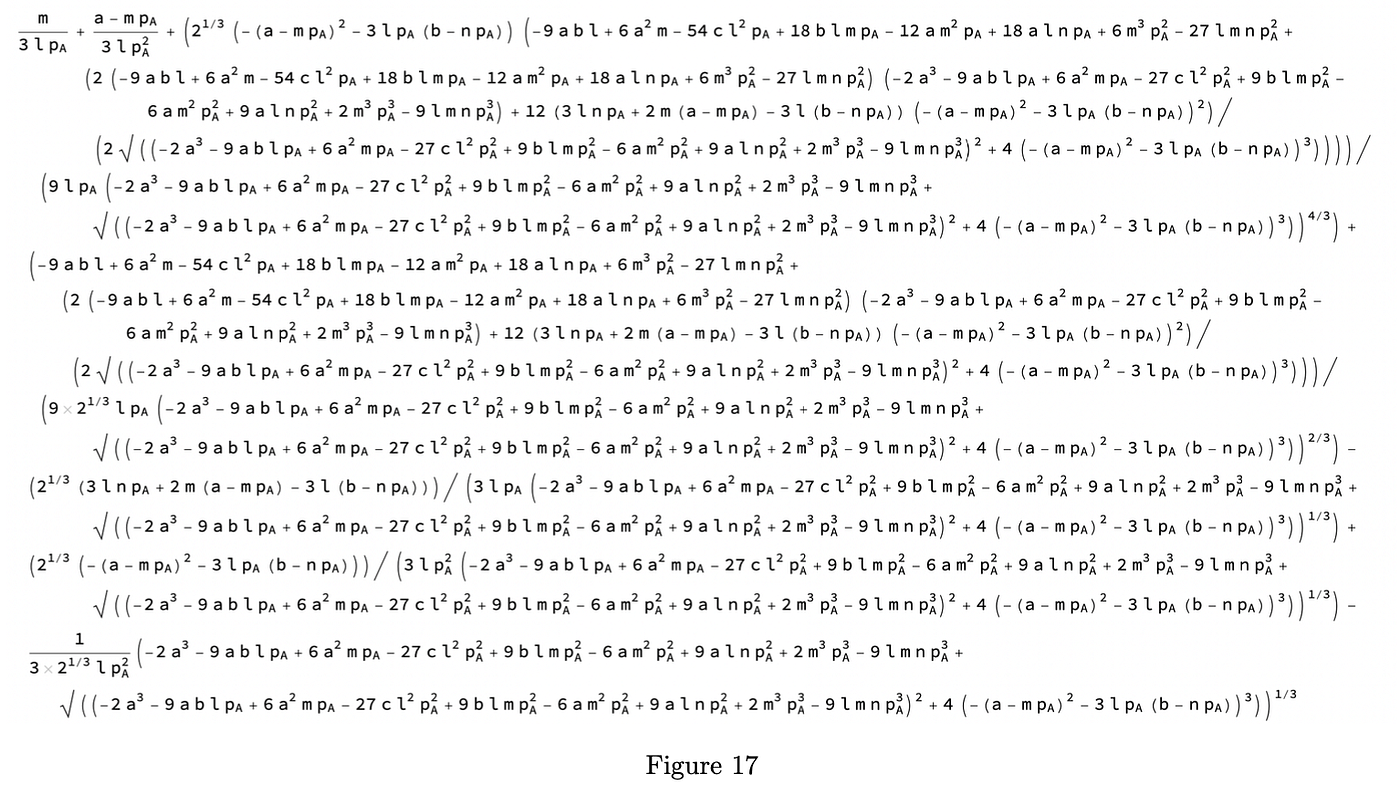
For liquidity density function

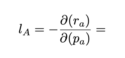
(13)

Reproduce of StableSwap[5]**

A more detailed analytical analysis is beyond the scope of this paper. However, we can set specific parameters³ to reproduce a stable swap mechanism as an example:

(14)

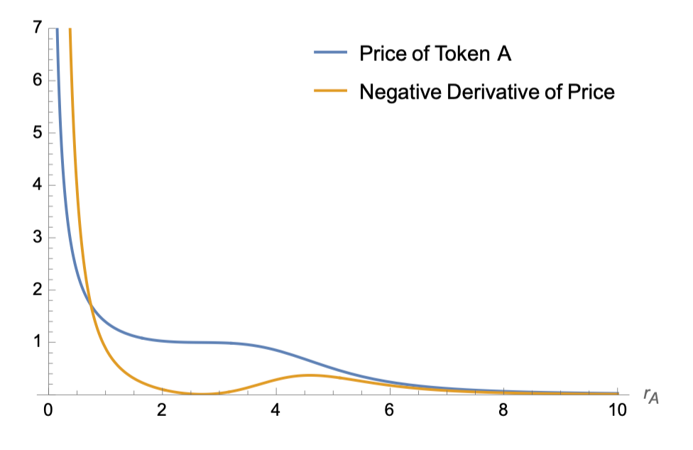
Figure 18: Bonding Curve

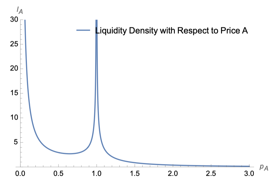
Figure 19: Liquidity Density Function

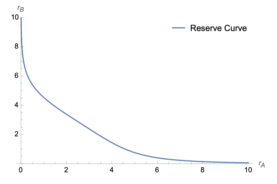
Figure 20: Reserve Curve

³ In models such as Curve, the parameter A needs to be dynamically adjusted according to liquidity depth changes, and D must be calculated iteratively during swaps. In contrast, our approach does not require such adjustments, as both A and D can be represented by constant values.

2.5 Prediction Markets

Prediction markets, also known as betting markets, information markets, decision markets, idea futures, or event derivatives, are open markets that enable the prediction of specific outcomes using financial incentives. In traditional bookmaker systems, such as horse racing betting, a centralized entity (the bookmaker) sets the odds and accepts bets from participants. While this system allows for flexible betting, it relies heavily on the centralized entity to manage the market, set odds, and handle payouts.

Overcoming Limitations with Bonding Curves By employing bonding curves, prediction markets can overcome these limitations and eliminate the need for a centralized bookmaker. Bonding curves provide a mathematical approach that allows for the issuance and redemption of tokens independently, without the necessity of matching buyers and sellers for each outcome at the same time. This flexibility enhances liquidity and enables participants to express their beliefs about future events more freely.

Traditionally, bonding curves define the relationship between the supply of a token and its price. However, this concept can be extended to represent the relationship between the supply of tokens and the reserve, effectively creating a supply-reserve function. In the context of prediction markets, the total reserve R can be expressed as a function of the supplies of the outcome tokens, allowing the market to adjust dynamically without centralized control.

Mathematical Representation and Reserve-Supply Relation

In the context of prediction markets, we can consider a bonding curve*[6]* that defines the relationship between the reserve of token B and supplies of tokens of different outcomes as:

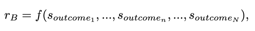
where r_B is the reserve of token B, s_outcomen is the supply of token for outcome n. An example⁴ of such a bonding curve for a two-outcome market (YES and NO) is:

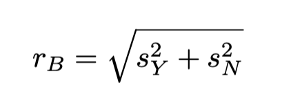
By using this reserve-supply function, the market can dynamically adjust the prices of outcome tokens based on their supplies and the total reserve. Participants can buy or sell tokens for any outcome independently, and the bonding curve ensures that prices reflect the current state of the market. This approach eliminates the need for issuing equal numbers of tokens or requiring simultaneous matching of buyers and sellers, as is necessary in some traditional prediction markets.

Figure 21: Illustration of the Bonding Curve for two-outcome prediction markets, linking the supplies of YES and NO tokens to the total reserve.

⁴ Still, many functional forms are possible, each representing different trade-offs between parameters. Another example can be r_B = b · ln(e^s_Y/b+e^s_N/b)

Token Purchase Mechanics In the bonding curve model, the price p(s_A) of a token is a function of its total supply s_A. A simple quadratic bonding curve can be expressed as:

(15)

This ensures that each token purchased reflects the current supply and its effect on the price, and the price will approach to 1 asymptotically when the market prefer outcome yes unidirectionally.

When a participant wishes to purchase an additional ∆_s yes tokens, the total cost C is calculated by integrating the price function over the desired token quantity:

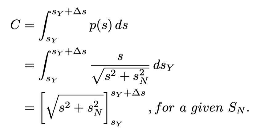
(16)

2.6 Time-dependent Bonding Curves

The bonding curve can be also include external parameter like time as:

Token Launch with Parameter time In the bonding curve model, the price p(s_A) of a token is a function of its total supply s_A. A simple quadratic bonding curve can be expressed as:

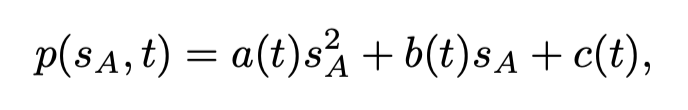
(17)

where a, b, and c are constants chosen to shape the curve appropriately. When a participant wishes to purchase an additional ∆_s tokens, the total cost C is calculated by integrating the price function over the desired token quantity:

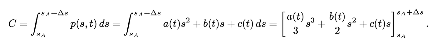
This ensures that each token purchased reflects the current supply and its effect on the price, accounting for the price increase as the total supply grows and vary as the time changes

Figure 22: 3D Plot of the Time-Dependent Bonding Curve p_A(s_A,t) = (1−t)(4s_A² + 6s_A) + 3, illustrating how the price of Token A varies with time and its supply.

Liquidity Bootstrapping Pool

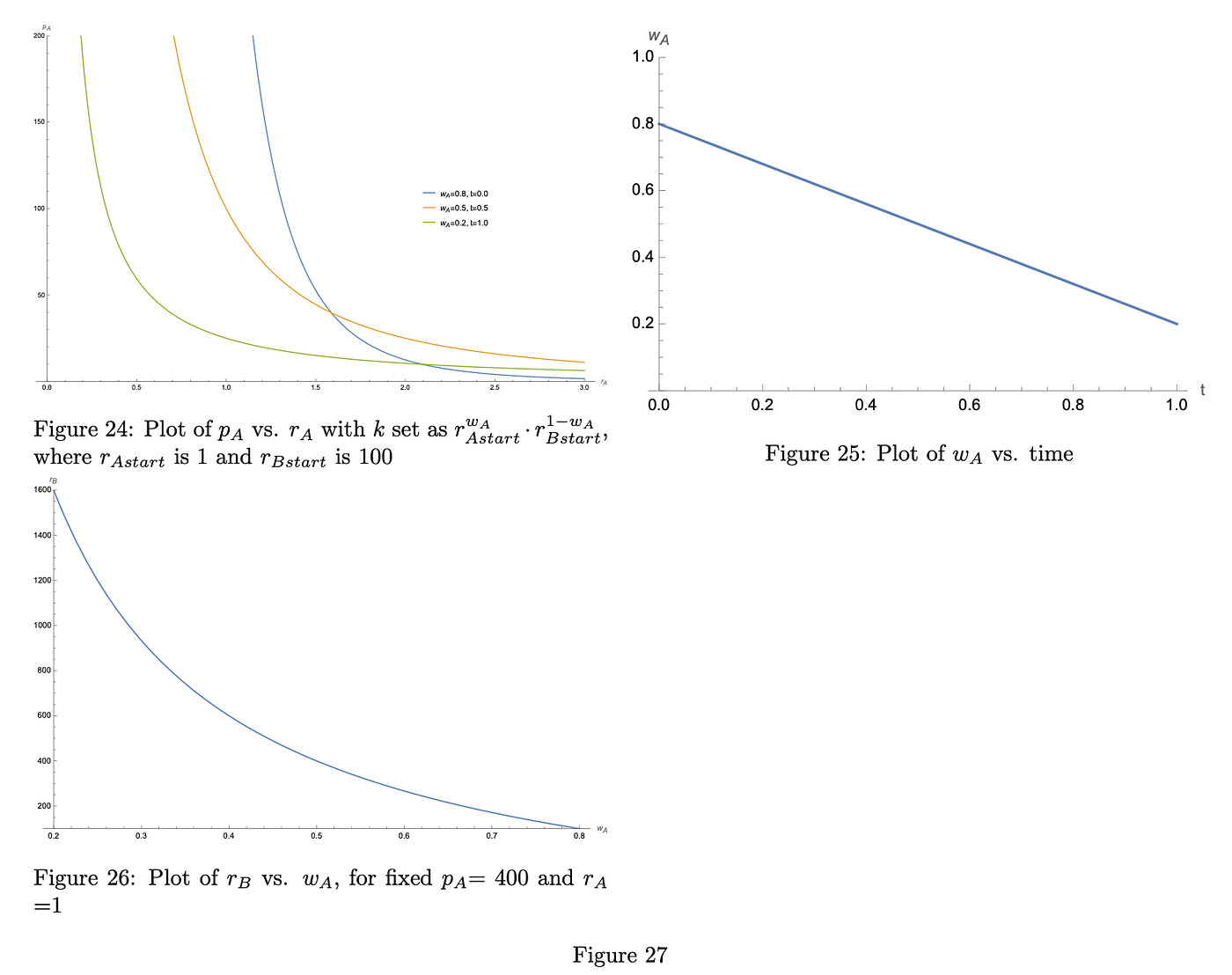
As another example, let us investigate liquidity bootstrapping pool. The core mechanism of an LBP involves starting with a high token price that gradually decreases over time unless buying pressure increases the price. This is achieved by adjusting the weights of the assets in the pool. For example, an LBP might begin with a high weight on the project’s token and a lower weight on a stablecoin or other counter asset. As time progresses, the weights adjust, causing the token’s price to decrease if there’s no buying pressure, encouraging participation and investment. LBPs facilitate price discovery by demonstrating the acceptable current price of an asset. Ideally, LBPs will have very few buyers at the time of launch. The price slowly declines until traders are willing to step in and buy the asset. An example of LBP is given by:

(18)

where w_A(t) is time-dependent explicitly and k is time-dependent implicitly.

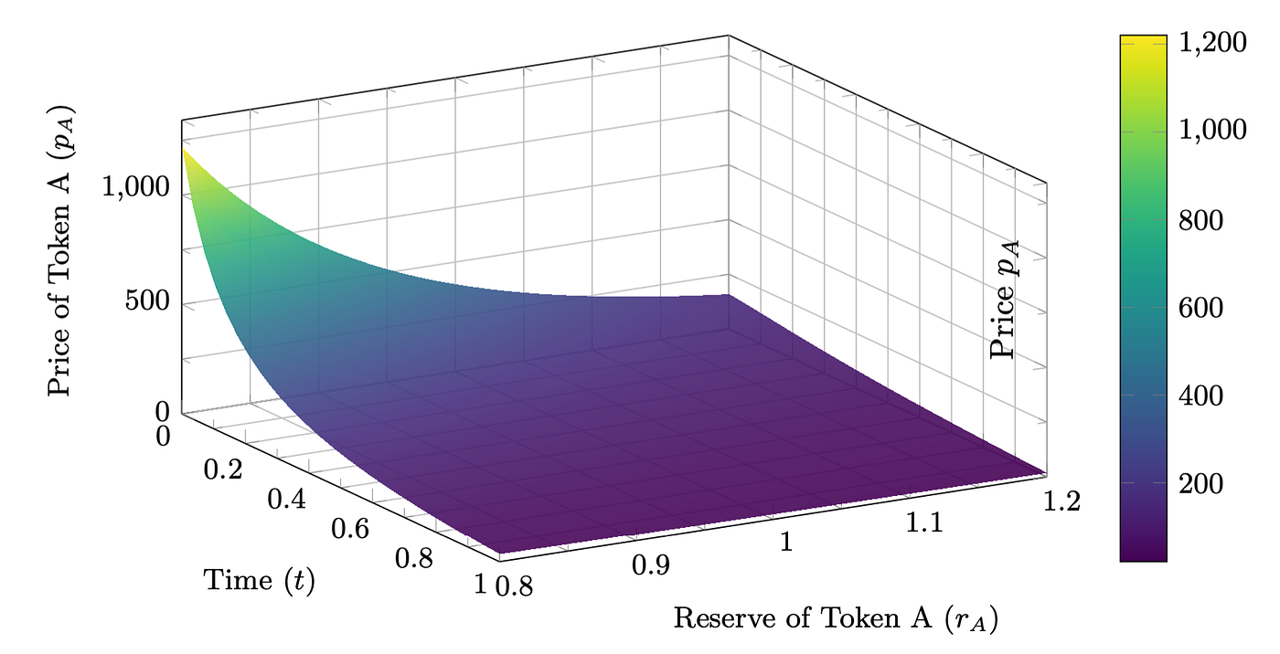
Figure 23: 3D Plot of the Price Function p_A(t,r_A) illustrating how the price of Token A varies with time and its supply.

2.7 Lending Market

The core function of the Bonding Curve in decentralized lending markets is to dynamically match loan demand and borrowing demand, automatically discovering the market’s risk preference to determine appropriate Loan-to-Value Ratio(LTV). Borrowers can set parameters such as token quantity, price range, interest rate, and liquidation ratio to create a lending curve that ensures flexible risk management and liquidity. This mechanism is not only suited for stable assets but also adapts well to volatile assets, addressing risk from price fluctuations and optimizing capital efficiency while enhancing the market’s inclusiveness.

Lending Curve

The black line represents the lending curve established by the borrower. In the diagram, this curve illustrates the lending price for ABC, where 0.5 signifies the minimum amount available for lending at a rate of 0.5 USDT/ABC, and 0.7 indicates the maximum amount available for lending at a rate of 0.7 USDT/ABC.

Lending Position

When the lender provides funds, a lending position will be created. Early participants benefit from lower lending prices(indicating how much can be borrowed per unit of collateral), while later participants face higher lending prices. Early positions have a lower risk of liquidation, making them suitable for investors seeking stable returns. In contrast, later positions have a higher risk of liquidation, allowing investors to potentially profit from liquidation events.

Figure 28: Lending curve

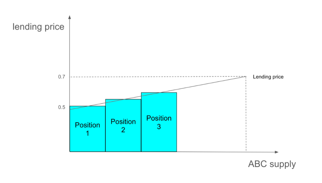
Figure 29: Positions on lending curve

Interest Accumulation

Interest will be accumulated separately based on the time of position creation, meaning that each lending position will accrue interest independently from others.

Figure 30: Interest Accumulation

Liquidation Process

When the user’s collateral value is insufficient to cover the principal and interest of the loan, the liquidation process will be triggered automatically.

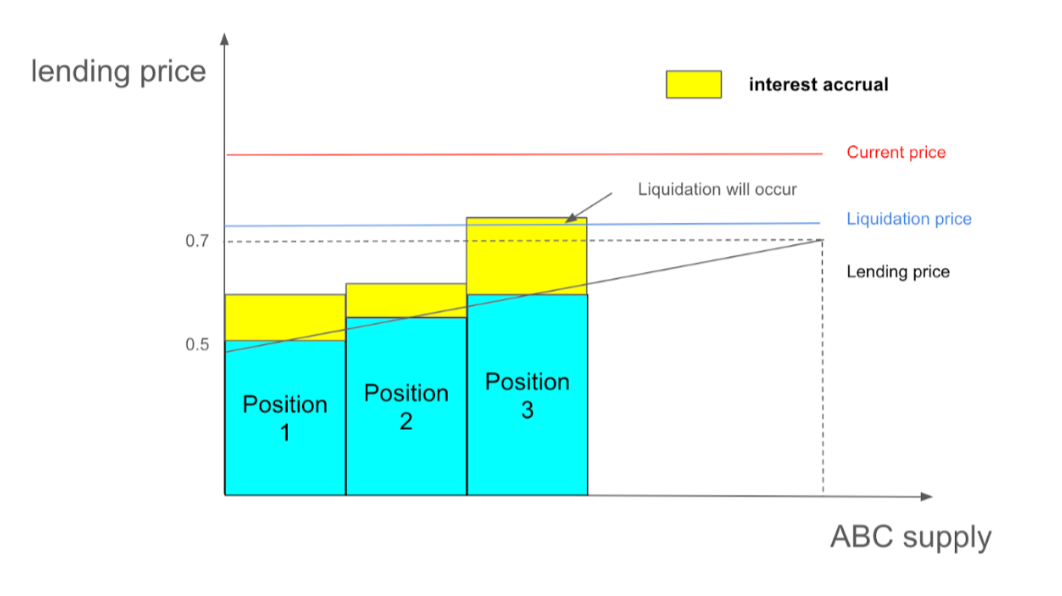
Figure 31: Liquidation Process

2.8 DAO Voting Systems

In broader decentralized applications, Decentralized Autonomous Organizations (DAOs) play a crucial role in gov-ernance. DAOs allow community members to participate in decision-making processes through a transparent andautomated system. Bonding curves can be innovatively applied to these voting systems to enhance their effectiveness and fairness.

Application of Bonding Curves in DAO Voting

Bonding curves can be utilized to manage voting power in DAOs. By linking the amount of tokens held to voting power via a bonding curve, these systems can discourage disproportionate influence by large token holders while encouraging wider participation from smaller stakeholders.

Mathematical Representation

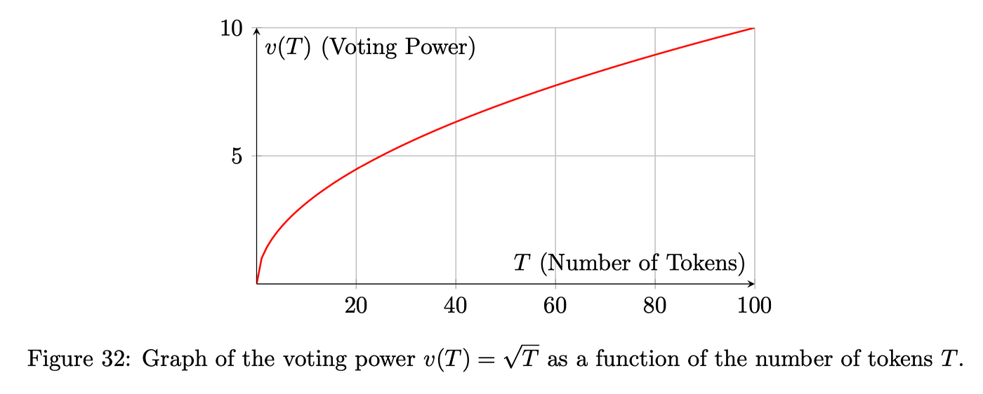
Let v(T) represent the voting power granted to a stakeholder as a function of the number of tokens T they hold. A bonding curve for this purpose might be defined as:

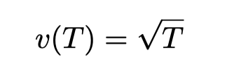
This square root function is selected because it provides diminishing returns on voting power as the number of tokens increases. This means that while increasing one’s token holdings still leads to more voting power, the rate of increase in power slows down significantly, preventing too much power from being concentrated with a single voter.

Benefits

Implementing a bonding curve in DAO voting offers multiple benefits:

Fairness: The square root curve reduces the gap between large and small token holders, promoting a more egalitarian approach to governance where decisions are less likely to be dominated by a few wealthy individuals.
Inclusivity: By diminishing the marginal increase in voting power, smaller stakeholders are encouraged to participate, knowing that their votes have a meaningful impact.
Scalability: As the organization grows, the bonding curve can be adjusted to maintain balance in voting power distribution, ensuring that the governance mechanism scales effectively with the size of the DAO.

2.9 Smart Society: Resource Allocation via Bonding Curves

In the context of a smart society, bonding curves can extend beyond traditional financial applications to encompass resource management and allocation. This innovative approach can effectively address common societal challenges, such as the sustainable management of natural resources. For instance, bonding curves can be employed to regulate fishing quotas based on the fish population in a river, thereby ensuring ecological balance and sustainable fishing practices.

Application of Bonding Curves

In the case of managing fish populations, a bonding curve can be designed to dynamically adjust fishing quotas based on real-time data regarding fish populations. This method not only provides a direct mechanism for controlling the extraction of resources but also incentivizes responsible behavior among stakeholders.

Mathematical Representation

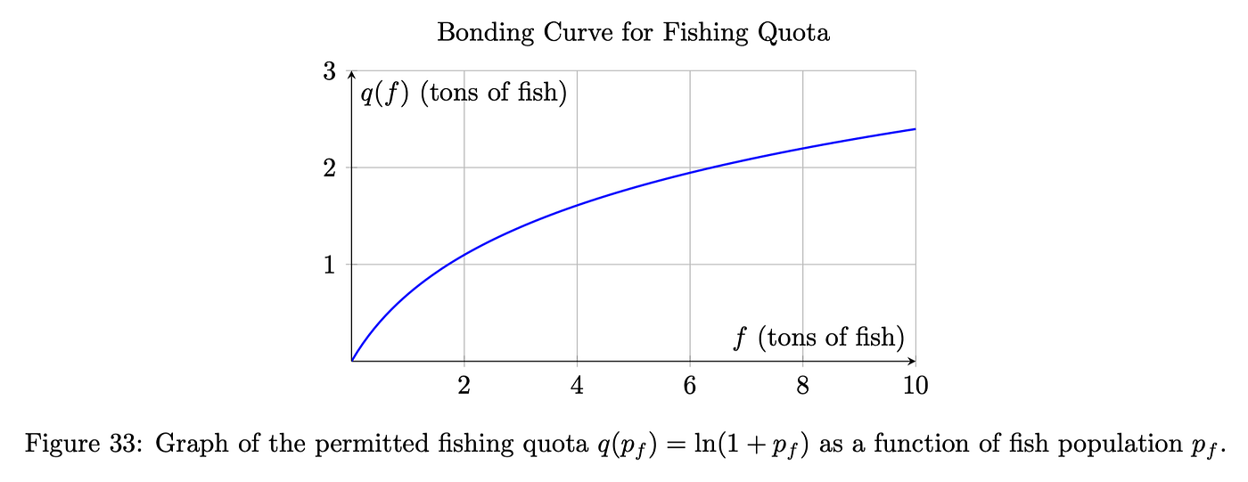
Let q(f) represent the permitted fishing quota (in tons of fish) as a function of the current fish population f in the river (measured in thousands of fish). The bonding curve can be expressed as:

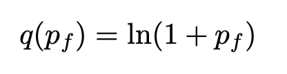
This logarithmic function is chosen because it increases gradually as the fish population grows, providing quotas that increase at a diminishing rate. This prevents excessive fishing when the population is vulnerable and allows more fishing as the population stabilizes and grows. The function’s responsiveness to smaller population sizes is crucial for preventing overfishing and promoting sustainable practices.

Benefits

The application of bonding curves in this manner offers several advantages:

Sustainability: Encourages sustainable fishing practices by directly linking fishing quotas to fish population levels.
Adaptability: Allows for dynamic adjustments in real-time, promoting quick responses to ecological changes.
Transparency: Provides a clear and transparent mechanism for stakeholders, reducing potential conflicts and improving compliance.

3 Mathematics Model

3.1 How to build a DeFi Protocol systematically

The design of a DeFi protocol involves a systematic approach that incorporates strategic planning and mathematical rigor. Below is the detailed process:

Define the Objective: Clearly identify the primary goal or function of the protocol, such as liquidity provision, trade facilitation, lending, or any other financial service. This initial clarity is crucial for aligning all subsequent design elements.
Identify the Participants: Determine the participants in the protocol, including traders, liquidity providers, borrowers, lenders, stakeholders, etc. Understanding their roles and requirements is essential for creating a fair and functional system.
Establish Bonding Curves: Determine if the main objective can be represented as an explicit or implicit function of other parameters. This step involves formulating mathematical models that depict how changes in one variable affect others, ensuring predictable and intended behavior under various scenarios.
Incentives and Disincentives: Create mechanisms that promote beneficial behaviors and discourage detri-mental actions within the protocol. This may include rewards for participation, transaction fees, penalties for malicious activities, and other regulatory measures to ensure the integrity and security of the protocol.
Implement the Input/Output Relations via Smart Contracts: Develop smart contracts to enforce the in-put and output relationships derived from the bonding curves. These contracts automate the protocol operations, ensuring they execute precisely as designed without the need for intermediaries.

3.2 Generalized Bonding Curve as Hypersurface

Consider the following system of equations governing the dynamics of the bonding curve:

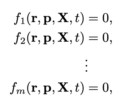
(19, 20, 21, 22)

where:

r = (r_1,r_2,…,r_n) represents the vector of token reserves.
p = (p_1,p_2,…,pn) denotes the vector of prices associated with these tokens.
X = (X_1,X_2,…,X_n) denotes the vector of parameters like fee, interest rate, fishing quota, reputation or whatever related.

For changes in the system, define:

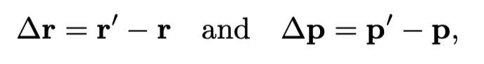
where:

r′= (r′_1,r′_2,…,r′_n) represents the updated vector of token reserves.
p′= (p′_1,p′_2,…,p′_n) denotes the updated vector of prices associated with these tokens.
X′ = (X′_1,X′_2,…,X′_n) denotes the vector of parameters like fee, interest rate, fishing quota, reputation or whatever related.
t′ is the updated time variable.

The dynamics of the bonding curve can be conceptualized as a walk on a hypersurface defined by the above equations. Although it is not feasible to explicitly express the input and output of tokens, we can calculate these changes. Even without an explicit expression, asymptotic analysis allows us to understand the system’s behavior, thereby clarifying the underlying arguments.

3.3 Optimal Targets through Lagrange Multipliers

To fine-tune the shape of the hypersurface representing the bonding curve, we aim to optimize the coefficients or parameters *X = (X_1,X_2,…,X_n)*. This optimization ensures that the hypersurface aligns with desired properties or performance metrics of the system. We employ the method of Lagrange multipliers to achieve this, considering the constraints defined by the bonding curve equations.

3.3.1 Formulating the Optimization Problem

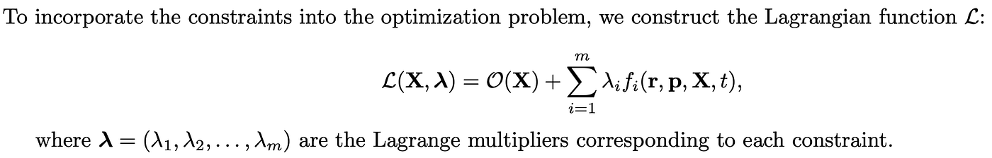
Assume we wish to optimize the parameters X to minimize a cost function *C(X)*, which could represent deviation from desired performance metrics, system stability measures, or any other relevant criteria. The optimization is subject to the bonding curve constraints:

(23, 24, 25, 26)

3.3.2 Constructing the Lagrangian

3.3.3 Deriving the Optimality Conditions

To find the optimal parameters X^∗, we take the partial derivatives of the Lagrangian with respect to each parameter X_j and the Lagrange multipliers λ_i, and set them to zero:

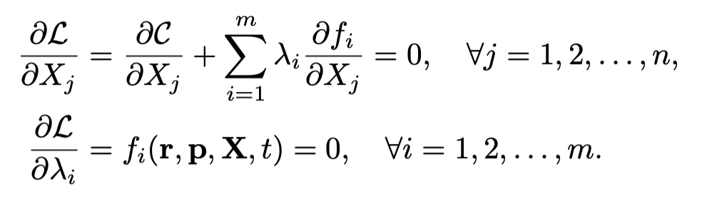
(27, 28)

These equations form a system of n+ m equations that can be solved simultaneously to determine the optimal parameters X^∗ and the corresponding Lagrange multipliers *λ^∗*.

3.3.4 Asymptotic Analysis

In scenarios where the system is too complex for closed-form solutions, asymptotic analysis can be employed to approximate the optimal parameters. By analyzing the behavior of the system as certain parameters X_j become large or small, we can derive approximate solutions that offer valuable insights into how to adjust the hypersurface’s shape effectively.

3.3.5 Practical Considerations

Parameter Sensitivity: Understanding which parameters Xj most significantly impact the hypersurface’s shape can guide targeted adjustments for optimal performance.
Computational Methods: Numerical optimization techniques, such as gradient descent or Newton-Raphson methods, may be necessary to solve the optimality conditions, especially in high-dimensional parameter spaces.
Constraint Qualification: Ensuring that the constraints satisfy regularity conditions (e.g., linear indepen-dence) is crucial for the validity of the Lagrange multiplier method.

3.3.6 Example

The Objective Function is:

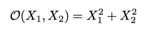
This is the function we want to minimize with respect to X_1 and X_2, subject to the constraints. The constraints are given by:

These constraints describe relationships between the reserves r, prices p, time t, and the parameters X_1 and X_2.

where X_1 and X_2 are the parameters to optimize, and λ_1 and λ_2 are the Lagrange multipliers corresponding to the constraints.

Deriving the Optimal Conditions: To find the optimal parameters X_1^∗ and X_2^∗ , we take the partial derivatives of the Lagrangian with respect to each parameter and the Lagrange multipliers, and set them to zero:

Solving this system of equations yields the following optimal parameters and Lagrange multipliers:

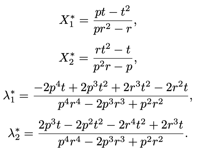
These are the optimal values of the parameters X_1^∗ and X_2^∗ that shape the function, and the corresponding Lagrange multipliers λ_1^∗ and *λ_2^∗*.

Interpreting the Results: The solutions X^∗ represent the set of parameters that best shape the hypersurface to meet the optimization criteria. The Lagrange multipliers λ^∗ provide insights into how sensitive the objective function is to each constraint, indicating the degree to which each bonding curve equation influences the optimization outcome. We need integrate out r and p to get the specific X^∗ and *λ^∗*.

4 Advanced Considerations in Bonding Curves

This section explores advanced aspects of bonding curves, focusing on Miner Extractable Value (MEV) attacks, precision processing combined with code efficiency, and practical applications of hypersurfaces in modeling bonding curves.

4.1 MEV Attacks in Bonding Curves

Miner Extractable Value (MEV) represents the additional profit that miners or validators can obtain beyond standard rewards by manipulating the ordering of transactions within blocks. In decentralized finance (DeFi) and bonding curves, MEV poses significant risks by enabling malicious actors to exploit transaction sequencing for personal gain, potentially undermining the system’s integrity and fairness. Bonding curves are particularly susceptible to strategies such as front-running, where miners prioritize their own transactions to benefit from anticipated price movements dic-tated by the bonding curve. Additionally, sandwich attacks allow miners to place buy and sell orders around a victim’s transaction to manipulate prices and extract value. Large transactions can also shift the bonding curve’s price, enabling miners to execute profitable trades before and after such changes. To mitigate these risks, several approaches can be implemented. Commit-reveal schemes separate transaction initiation and execution phases, reducing predictability and making it harder for miners to front-run. Batch auctions execute multiple transactions simultaneously at a single clearing price, minimizing MEV opportunities. Randomized transaction ordering introduces unpredictability in trans-action sequencing, disrupting predictable exploitation. Additionally, utilizing private or off-chain transaction pools can obscure transaction details from miners until execution, further reducing MEV risks.

4.2 Precision Processing and Code Efficiency

Accurate computation and optimized code are critical in bonding curves to ensure price stability, fairness, and security. Moreover, in blockchain-based implementations, efficient code is essential to minimize gas costs, making the system more sustainable and cost-effective for users. Maintaining precision in bonding curves involves overcoming challenges such as floating-point errors, which can introduce rounding inaccuracies in iterative calculations. Handling large-scale calculations with extremely large or small numbers exacerbates precision issues, especially within the constraints of smart contracts that have limited computational precision and incur high gas costs. To address these challenges, fixed-point arithmetic can be employed to provide consistent precision with lower computational overhead. Optimized algorithms that reduce computational complexity help in minimizing gas consumption without sacrificing accuracy. Normalization techniques, which scale numbers to maintain precision, further enhance computational reliability. Regu-lar code auditing and validation are also essential to ensure that smart contracts maintain both precision and efficiency, safeguarding against potential vulnerabilities.

4.3 Practical Cases for Hypersurfaces

Hypersurfaces enable the modeling of multidimensional relationships in bonding curves, facilitating the representation of interactions within multi-token ecosystems. They allow for dynamic parameter adjustments, such as adapting fees, interest rates, and quotas based on the system’s current state. Additionally, hypersurfaces support scenario analysis by visualizing the impact of changes in one dimension on others, aiding in comprehensive system evaluation. For instance, a decentralized exchange (DEX) utilizing a bonding curve for liquidity provision can model various dimensions including token reserves, token prices, system parameters like trading fees and slippage tolerance, and temporal dynamics affecting supply and demand. This multidimensional modeling allows the DEX to optimize liquidity provision, maintain price stability, and adapt dynamically to changing market conditions, enhancing overall system performance. Similarly, Automated Market Makers (AMMs) like Uniswap leverage bonding curves to facilitate token swaps without traditional order books. Hypersurfaces aid in liquidity optimization by balancing reserves and fees to enhance liquidity while reducing impermanent loss. They also enable the implementation of dynamic fee structures that adjust based on trading volume or market volatility. Furthermore, hypersurfaces facilitate the management of multiple liquidity pools within a unified framework, allowing for efficient multi-pool interactions. Visualizing high-dimensional hypersurfaces presents challenges, but techniques such as dimensionality reduction, contour mapping, and interactive 3D models can aid in interpretation. These methods help developers and analysts comprehend complex system behaviors, identify optimal parameter settings, and predict responses to market changes, thereby facilitating effective system optimization and decision-making. In summary, hypersurfaces provide a robust framework for modeling and optimizing complex, multidimensional bonding curve systems, enhancing their performance, stability, and adaptability in dynamic market environments.

5 Conclusion

In this paper, we have meticulously explored the versatility and potential of bonding curves as a foundational tool for constructing a wide array of Decentralized Finance (DeFi) protocols. By extending the traditional application of bonding curves beyond Automated Market Makers (AMMs), we demonstrated their capability to underpin diverse financial mechanisms, including fair launches, token swaps, prediction markets, loan markets, DAO voting systems, company equity distribution, futures contracts, stablecoin design, and even resource allocation in smart societies.

References

[1] Lucius Fang, Erina Azmi, Benjamin Hor, Khor Win Win, et al. How to DeFi: Advanced, volume 1. CoinGecko,2021. [2] Simon de la Rouviere. Tokens 2.0: Curved token bonding in curation markets. Medium, 2017. [3] Michael Zargham, Jamsheed Shorish, and Krzysztof Paruch. From curved bonding to configuration spaces. In 2020 IEEE International Conference on Blockchain and Cryptocurrency (ICBC), pages 1–3. IEEE, 2020. [4] Hayden Adams, Noah Zinsmeister, Moody Salem, and Daniela Robinson. Uniswap v3 core. https://api.semanticscholar.org/CorpusID:232416764, 2021. Accessed: 2024–10–12. [5] Michael Egorov. Stableswap-efficient mechanism for stablecoin liquidity. Retrieved Feb, 24:2021, 2019. [6] Obyte. Introducing prophet: Prediction markets based on bonding curves. https://blog.obyte.org/introducing-prophet-prediction-markets-based-on-bonding-curves-3716651db344, 2019. Accessed: 2024-10–12.

PDF: [Bonding Curves: A Universal Tool for Building DeFi Protocols]